American sports fans love numbers. Europeans are all vibes. Fighting and vibes. The American Soccer1 Revolution of the late ’00s and early ’10s brought a sea of nerds armed with calculators, ready to formalise the sport with mathematical proofs. So came the birth of a new era of football, where we rid ourselves of the shackles of Actually Watching Games and studied the sport in its purest form, the spreadsheet.
Analytics has become a permanent fixture in football, with every club having teams of analysts to scout players and opponents and measure performance. Metrics like expected goals (xG) are increasingly common in football media coverage. America’s finest nerds have spent years devising ways to explain this silly little sport to the unwashed European masses, including leaning on existing concepts and ideas in American sports to build metrics that help explain football in valuable ways.
However, a standard metric that has remained relatively untouched is the strength of schedule (SOS). SOS measures the quality of the opponents a team has faced or will face to account for the difficulty of a team’s schedule when judging past performances or predicting future outcomes.
While SOS is less useful in European sports, where leagues are generally structured so that every team has an equal schedule, it can still be helpful when trying to say meaningful things about what has or will happen, both in domestic leagues and continental (and international) knockout tournaments.
I will develop a simple method for measuring SOS that can be easily implemented and interpreted. I hope my ideas become pervasive like the American Soccer Nerds all around us.
A Simple Approach to Measuring Schedule Strength
My goal with developing an SOS metric for football is to create something relatively simple but still does a solid job of capturing schedule difficulty. I’m sure there will be more precise ways to get at this, but I want to maximise the precision while maintaining simplicity in both implementation and interpretation. For something like this, a decent metric that is really easy to use is much better than a really accurate metric that is particularly complex for anyone looking to use or understand it.
The simplest approach to measuring schedule difficulty is to use the winning record of a team’s opponents to capture how well the team’s opponents have been doing in the league that season. For example, the Wikipedia entry for Strength of Schedule lists the following formula:
\[SOS = \frac{2(OR) + (OOR)}{3}\] where OR is the opponents’ winning record, and OOR is the opponents’ opponents winning record. There are many variants to this, some more complex than others2, but the fundamental issue with this approach is that wins and losses are all counted equally. A win over some garbage team (for example, Portsmouth FC) means just the same as a way against a heavyweight (for instance, Southampton FC). I like the approach to capturing the inequality in the quality of the teams that a team’s opponents have played, but the issues with using winning records are insurmountable.
Calculating Baseline Team Ratings
Instead, measuring the difficulty of a team’s schedule should start with making at least a half-decent effort to quantify each opponent’s strength. I will calculate a relatively crude measure of baseline team ratings using non-penalty goal difference per 90 (npG/90) and non-penalty expected goal difference per 90 (npxGD/90)3.
I will take a weighted combination of npxGD/90 (70%) and npGD/90 (30%) because previous work suggests this is the optimal way to combine the two (Torvaney 2021a).
This approach benefits from conceptual simplicity, making for a relatively straightforward interpretation.
Estimating Home Advantage
Rather than making wild assumptions about home advantage, I decided to do the responsible thing: measure the average home advantage across the big five leagues in recent seasons and use that number to weight home games.
I used the excellent worldfootballR package to grab match results data in the big five leagues from 2017/18 to 2022/23 from FBref focusing on actual and expected goals (because penalties are relevant when measuring home advantage). I have also dropped any rows where attendance is NA, assuming that NAs represent empty stadiums, particularly during the COVID-19 pandemic.
Table 1 shows the league average percentage difference in goals scored by home teams compared with away teams, and the average for the big five leagues is calculated, too.
Table Code (Click to Expand)
home_and_away |> tidyr::drop_na() |>bind_rows( home_and_away |>summarise(across(ends_with("_goals") |ends_with("_xg"), mean) ) |>mutate("league"="Big Five Leagues") ) |>summarise(across(ends_with("_goals") |ends_with("_xg"), mean),.by =c(league) ) |>mutate(goal_diff = (home_goals - away_goals) / away_goals,xg_diff = (home_xg - away_xg) / away_xg ) |>select(league, goal_diff, xg_diff) |>rename("League"="league","Goals"="goal_diff","Expected Goals"="xg_diff" ) |>gt() |>tab_spanner(label ="Difference (Home vs Away)",columns =2:3 ) |>tab_footnote("Excluding games played without fans in attendance.") |>tab_style(style =list(cell_text(weight ="bold")),locations =cells_body(columns =everything(),rows = League =="Big Five Leagues" ) ) |>tbl_theme(type ="pct", .round =1)
Table 1: Average Home Advantage in the Big Five Leagues 2017/18 - 2022/23
League
Difference (Home vs Away)
Goals
Expected Goals
Premier League
26.6%
24.3%
La Liga
35.1%
34.8%
Ligue 1
28.7%
24.9%
Bundesliga
30.2%
24.6%
Serie A
17.8%
18.7%
Big Five Leagues
27.4%
25.3%
Source: FBref Via {worldfootballR}
Excluding games played without fans in attendance.
The variance in the percentage difference in both goals and expected goals in Table 1 is pretty high, though that does appear to be driven by Serie A and La Liga being at the extreme ends. The Premier League, Bundesliga, and Ligue 1 variance is significantly lower. This is interesting, but I will avoid going down this specific rabbit hole right now because rabbit hole inception is a step too far.
I’m doing my duty as a Brexit-era Englishman focusing only on English leagues and pretending that football does not exist outside these fair shores. Taking the average across the big five leagues is acceptable for these purposes. Although the average is just above 25% for both goals and expected goals, I’m not going to be an insufferable bore5. I will treat the home advantage as 25% to keep things simple.
Team ratings will be weighted by home advantage by adding 25% of the team rating’s absolute value to the rating.
Notation (Click to Expand)
\[
R_{ij} = \\
\begin{cases}
R_j + |R_j| \cdot H & \text{if game is at opponent's home} \\
R_j & \text{otherwise}
\end{cases}
\] where \(R_{ij}\) is the opponent team’s rating, \(R_j\) is their baseline rating (with \(|R_j|\) representing the absolute value of the opponent’s baseline rating), and \(H\) is the home advantage weighting.
Putting it All Together
We should now be able to assemble everything to create an SOS model.
The first step is to calculate the opponents’ ratings (OR) and the opponents’ opponents’ ratings (OOR)6. I will do this by first calculating the weighted team rating for each fixture, meaning that when a team plays away from home OR will be 25% higher and when they are at home, OOR is 25% higher. I will then take the mean value of OR and OOR. This second value is more involved, but it is conceptually the same as the mean value of OR.
Notation (Click to Expand)
\[ \hat{OR}_i = \frac{1}{n} \sum_{j=1}^n { R_{ij}^\prime } \] where \(\hat{OR}_i\) is the mean average opponents’ ratings for team \(i\), \(n\) is the total number of opponents that team \(i\) faces, and \(R_{ij}^\prime\) denotes the adjusted rating of opponent \(j\) when playing against team \(i\), accounting for the home advantage.
A similar process can also be carried out to calculate team \(i\)’s OOR (\(OOR_i\)). However, you have to calculate the ratings for each of team \(i\)’s opponents’ opponents, then take the mean average value for each opponent’s schedule, and then the mean average for all of team \(i\)’s opponents.
where \(\hat{OOR}_i\) represents the mean value of team \(i\)’s OOR, \(n\) is the total opponents, \(m_j\) is the total number of opponents for opponent \(j\) of team \(i\), and \(R_{jk}^\prime\) is the rating of opponent \(k\) when playing against opponent \(j\) of team \(i\).
The outer sum iterates over each opponent of team \(i\), and for each opponent \(j\), while the inner sum calculates the mean rating of their opponents (opponents of opponent \(j\)). Finally, the outer sum computes the mean value of these mean ratings over all opponents of team \(i\).
The average value of a team’s OR and OOR play slightly different roles in the model. OR is the model’s primary parameter, and OOR provides additional context, allowing us to weight OR by the quality of the opponents’ opposition.
I will take a weighted average of OR (66.6%) and OOR (33.3%) and sum the two values.
Notation (Click to Expand)
Using the values \(OR_i\) and \(OOR_i\), we can calculate the strength of schedule for team \(i\) by weighting the two ratings.
While this approach yields a defensible SOS metric, the interpretability of the results may be limited. I have concerns about the practical significance of SOS values measured on the same scale as goals per 90. What does it mean for a team to have a one-goal-per-90 advantage in SOS? Are unit increases and decreases in SOS linear across the range of values? I think using the same scale as goals per 90 may lead to oversimplification and potential misinterpretation of SOS values7.
Instead, transforming SOS onto a standard scale, such as z-scores, offers a solution. Z-scores provide a standardised measure that facilitates precise comparative analysis across teams or seasons. This approach makes the results easier to interpret and allows for more meaningful comparisons within the league context.
SOS z-scores are calculated by taking the mean average and standard deviation of SOS for the entire league. For each unstandardised value of SOS, we subtract the mean and divide the result by the standard deviation.
Notation (Click to Expand)
\[ SOS_i^\prime = \frac{SOS_i - \mu_{SOS}} {\sigma_{SOS}} \] where \(SOS_i^\prime\) is the standardised SOS z-score for team \(i\), while \(\mu_{SOS}\) is the mean value of all SOS and \(\sigma_{SOS}\) is the standard deviation of all SOS.
An SOS that equals zero is a league-average schedule; scores greater than zero are harder than the league average, and scores less than zero are easier than the league average. If a team’s SOS z-score is +1, their SOS is one standard deviation above the average SOS for all teams. Similarly, a z-score of -1 indicates that the SOS is one standard deviation below the average. Z-scores allow us to compare different teams’ SOS values on a standard scale, making it easier to interpret and analyse their relative strengths of schedule.
Premier League Strength of Schedule
The upside of Sunday’s dull 0-0 draw between Man City and Arsenal is that this was the ideal result for extending this incredible three-way title race in the Premier League. This is precisely the situation where a quantitative measure of the difficulty of each team’s schedule down the stretch would be valuable. Sounds like the perfect way to test this metric! I grabbed team-level goals and expected goals data and match results for the 2023/24 season in the Premier League from FBref via worldfootballR.
I have also turned all of this into an R package, fitba8. This should also make it easier for anyone to use this code and build on the method.
Remaining Schedule
The first step is to filter the match results data to only include the remaining games we want to work with. We can leverage that worldfootballR’s fb_match_results() function also includes future games with undetermined details about the match, like home and away goals, set to NA.
This creates a dataframe with every remaining fixture in the 2023/24 Premier League season repeated twice, with each team listed once in the team and opponent columns. Table 2, below, shows a sample of the data.
Table 2: Sample of Remaining Premier League Fixtures
Team
Home or Away
Opponent
Manchester Utd
Home
Liverpool
Bournemouth
Home
Crystal Palace
Manchester City
Away
Tottenham
Brentford
Away
Aston Villa
Crystal Palace
Home
Newcastle Utd
Everton
Home
Nott'ham Forest
Manchester City
Away
Brighton
Luton Town
Home
Fulham
Nott'ham Forest
Home
Manchester City
Liverpool
Home
Tottenham
Source: FBref Via {worldfootballR}
To me, this seems like the obvious way to structure the data, but it’s important to remember that I am an idiot, so there may well be a better way.
Baseline Team Ratings
The next step is to create the baseline ratings for each Premier League team using their npxGD/90 and npGD/90. As discussed in Section 1, calculating the team ratings is very simple. They are just a weighted average of npxGD/90 (70%) and npGD/90 (30%).
Table 3: Baseline Team Ratings in the Premier League
Team
npxGD/90
npGD/90
Rating
Arsenal
1.12
1.27
1.17
Manchester City
0.97
1.17
1.03
Liverpool
0.85
1.14
0.94
Tottenham
0.3
0.72
0.43
Aston Villa
0.21
0.53
0.31
Chelsea
0.34
−0.11
0.2
Brighton
0.17
0.11
0.15
Everton
0.23
−0.04
0.15
Newcastle Utd
0.08
0.28
0.14
Bournemouth
0.02
−0.25
−0.06
Brentford
0.07
−0.5
−0.1
Fulham
−0.27
0.2
−0.13
Manchester Utd
−0.29
0
−0.2
West Ham
−0.29
0
−0.2
Nott'ham Forest
−0.14
−0.43
−0.23
Wolves
−0.28
−0.14
−0.24
Crystal Palace
−0.26
−0.52
−0.34
Burnley
−0.72
−0.97
−0.79
Luton Town
−0.95
−0.73
−0.88
Sheffield Utd
−1.05
−1.69
−1.24
Source: FBref Via {worldfootballR}
According to Table 3, Arsenal are the best team in the league, which seems about right, followed by Manchester City and Liverpool, and then a giant chasm before we reach the rest of the league (which is topped by Tottenham). I am not compelled to argue with these ratings, but if you’re a Manchester United fan who doesn’t have the capacity for shame, you might?
We then have to calculate the mean rating for a team’s OR and OOR from these baseline ratings. The process for calculating each of these is similar. However, the home advantage weighting is reversed for the OOR, and a little extra work is required to get the opponents that a team’s opponents will face.
Table 4 shows the two sets of ratings joined by their corresponding team, which hopefully helps make sense of what is happening here. This part of the process is a little confusing because the steps are kind of stacked on top of each other. Fingers crossed, this makes it easier to follow.
Table Code (Click to Expand)
remaining_games |>distinct(team) |>arrange(team) |>left_join(opponent_ratings, by =join_by(team)) |>left_join(opponent_opponent_ratings, by =join_by(team)) |>rename("Team"= team,"Opponents' Rating"= opponent_rating,"Opponents' Oppponents Rating"= opponent_opponent_rating, ) |>gt() |>tbl_theme(type ="num")
Table 4: Team Opponents’ & Opponents’ Oppponents Ratings
Team
Opponents' Rating
Opponents' Oppponents Rating
Arsenal
0.01
0.17
Aston Villa
0.46
0.03
Bournemouth
0.08
0.15
Brentford
−0.15
0.13
Brighton
0.22
0.02
Burnley
−0.07
0.06
Chelsea
0.1
0.13
Crystal Palace
0.21
0.07
Everton
−0.02
0
Fulham
0.09
0.02
Liverpool
−0.14
0.16
Luton Town
0.28
0.03
Manchester City
−0.09
0.2
Manchester Utd
0.04
0.04
Newcastle Utd
−0.19
0.07
Nott'ham Forest
0.01
0.06
Sheffield Utd
0.1
−0.03
Tottenham
0.19
−0.01
West Ham
0.18
0.1
Wolves
0.15
0.05
Source: FBref Via {worldfootballR}
Strength of Schedule
Having created all the components needed, we must piece it together like a dullard’s jigsaw puzzle.
strength_of_schedule <- remaining_games |>distinct(team) |>left_join(opponent_ratings, by =join_by(team)) |>left_join(opponent_opponent_ratings, by =join_by(team)) |>mutate(unstandardized = (2/3* opponent_rating) + (1/3* opponent_opponent_rating),sos =scale(unstandardized) )
We can start by looking at the Premier League title race, comparing Arsenal, Manchester City, and Liverpool’s schedules. Table 5 shows the results.
Table Code (Click to Expand)
strength_of_schedule |>select(team, sos) |>filter(team %in%c("Arsenal", "Manchester City", "Liverpool")) |>arrange(sos) |>rename("Team"= team,"Strength of Schedule (Z-Score)"= sos ) |>gt() |>tab_footnote(footnote ="z < 0 = Easier than league average; z > 0 = Harder than league average" ) |>tbl_theme(type ="num")
Table 5: Premier League Title Race’s Strength of Schedule
Team
Strength of Schedule (Z-Score)
Liverpool
−1.12
Manchester City
−0.67
Arsenal
−0.09
Source: FBref Via {worldfootballR}
z < 0 = Easier than league average; z > 0 = Harder than league average
As discussed in Section 1.3, z-scores are a measure of standard deviation from the mean. A z-score of -1.12 means that Liverpool’s schedule is 1.12 standard deviations lower than the mean league schedule.
All three teams’ schedules are easier than the league average, which is unsurprising because they have played each other, and many teams still have to play them. However, there is plenty of variance in schedule strength between the three title contenders. Arsenal’s schedule is very close to the league average, while Liverpool’s remaining schedule is one of the easiest in the Premier League.
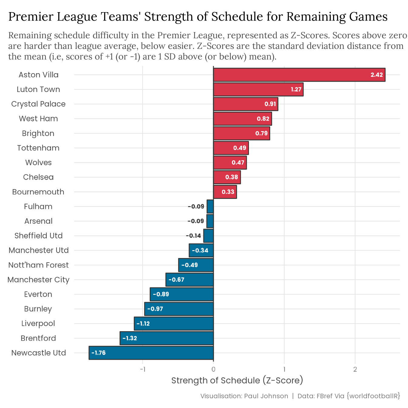
Finally, we can plot the Strength of Schedule Z-Scores for all Premier League teams’ remaining games this season. The plot below orders teams by SOS, from the hardest schedules to the easiest.
Plot Code (Click to Expand)
strength_of_schedule |>mutate(team = forcats::fct_reorder(team, sos)) |>ggplot(aes(x = team, y = sos, fill = sos >0)) +geom_col(colour ="grey20") +geom_hline(yintercept =0, colour ="grey20") +geom_text(aes(label =round(sos, 2),colour =between(sos, -0.25, 0.25),hjust =case_when(between(sos, -0.25, 0) ~1.2,between(sos, 0, 0.25) ~-0.4, sos <-0.25~-0.2, sos >0.25~1.2 ) ),size =5, fontface ="bold", family ="Poppins" ) +coord_flip() +scale_fill_manual(values =c("#026E99", "#D93649"), guide ="none") +scale_colour_manual(values =c("white", "grey20"), guide ="none") +labs(title ="Premier League Teams' Strength of Schedule for Remaining Games",subtitle = stringr::str_wrap( glue::glue("Remaining schedule difficulty in the Premier League, represented as ","Z-Scores. Scores above zero are harder than league average, below ","easier. Z-Scores are the standard deviation distance from the mean ","(i.e, scores of +1 (or -1) are 1 SD above (or below) mean)." ),width =95 ),x =NULL, y ="Strength of Schedule (Z-Score)",caption ="Visualisation: Paul Johnson | Data: FBref Via {worldfootballR}" )
Aston Villa and Luton have much left to play for, so this is not great news for either side. Meanwhile, Newcastle doesn’t have to face any of the top three but still have to play Sheffield United and Burnley. Their schedule includes only three teams ranked in the top ten in the baseline team ratings, two of which they will face at St James’ Park. Awful slackers.
Championship Strength of Schedule
We can take another look at this SOS model and how the fitba package I’ve put together works, using the race for automatic promotion in the Championship. As a Southampton fan, I am presenting this as a four-way race that includes Saints, despite their loss to Ipswich on Monday. This choice might seem a little unrealistic. However, I spent four years in a PhD program, so I’m excellent at convincing myself that everything is going great despite the crushing weight of evidence suggesting otherwise.
Table 6: Baseline Team Ratings in the Championship
Team
npxGD/90
npGD/90
Rating
Leeds United
0.82
0.95
0.86
Leicester City
0.67
0.77
0.7
Ipswich Town
0.6
0.88
0.68
Southampton
0.69
0.55
0.65
West Brom
0.19
0.52
0.29
Coventry City
0.24
0.39
0.28
Middlesbrough
0.3
0.08
0.23
Watford
0.14
0.18
0.15
Norwich City
0.02
0.37
0.12
Sunderland
0.16
−0.07
0.09
Hull City
0.03
0.08
0.05
Bristol City
−0.09
0.03
−0.05
Blackburn
−0.01
−0.18
−0.06
Stoke City
−0.08
−0.37
−0.17
Millwall
−0.19
−0.23
−0.2
Preston
−0.3
−0.07
−0.23
Swansea City
−0.26
−0.17
−0.23
QPR
−0.23
−0.38
−0.28
Sheffield Weds
−0.13
−0.63
−0.28
Huddersfield
−0.23
−0.53
−0.32
Plymouth Argyle
−0.41
−0.12
−0.32
Birmingham City
−0.37
−0.45
−0.39
Cardiff City
−0.55
−0.35
−0.49
Rotherham Utd
−1
−1.18
−1.05
Source: FBref Via {worldfootballR}
However, it is regrettable that my ratings are trying to convince me that Ipswich are good. Sure, they beat Southampton 3-2 on Monday. Still, Southampton were the (slightly) better team, and I watched Cardiff City dominate them earlier in the season, so I am convinced they are frauds that are going to Splendid Vibes their way to the Premier League10. Ipswich should be illegal.
Having calculated the (clearly wrong, disrespectful) team ratings, we can examine the schedules for the four teams left in the race for the automatic promotion spots. Table 7 shows the SOS for the Championship’s top four teams.
Table Code (Click to Expand)
champ_sos |>filter(team %in%c("Ipswich Town", "Leeds United", "Leicester City", "Southampton")) |>arrange(sos) |>rename("Team"= team,"Strength of Schedule (Z-Score)"= sos ) |>gt() |>tab_footnote(footnote ="z < 0 = Easier than league average; z > 0 = Harder than league average" ) |>tbl_theme(type ="num")
Table 7: Championship Promotion Race’s Strength of Schedule
Team
Strength of Schedule (Z-Score)
Leicester City
−0.28
Ipswich Town
0.45
Southampton
1.02
Leeds United
1.1
Source: FBref Via {worldfootballR}
z < 0 = Easier than league average; z > 0 = Harder than league average
If the now slim probability of automatic promotion wasn’t enough, Saints also face one of the most challenging schedules, only beaten by Leeds. Saint have to play Leeds and Leicester before the end of the season, both away from home, in addition to Coventry and Preston, who are still in the hunt for the final playoff spot. Southampton are the toughest team any of the others will face, though Leeds and Ipswich still have to face several playoff chasers, and Leicester are up against multiple relegation candidates.
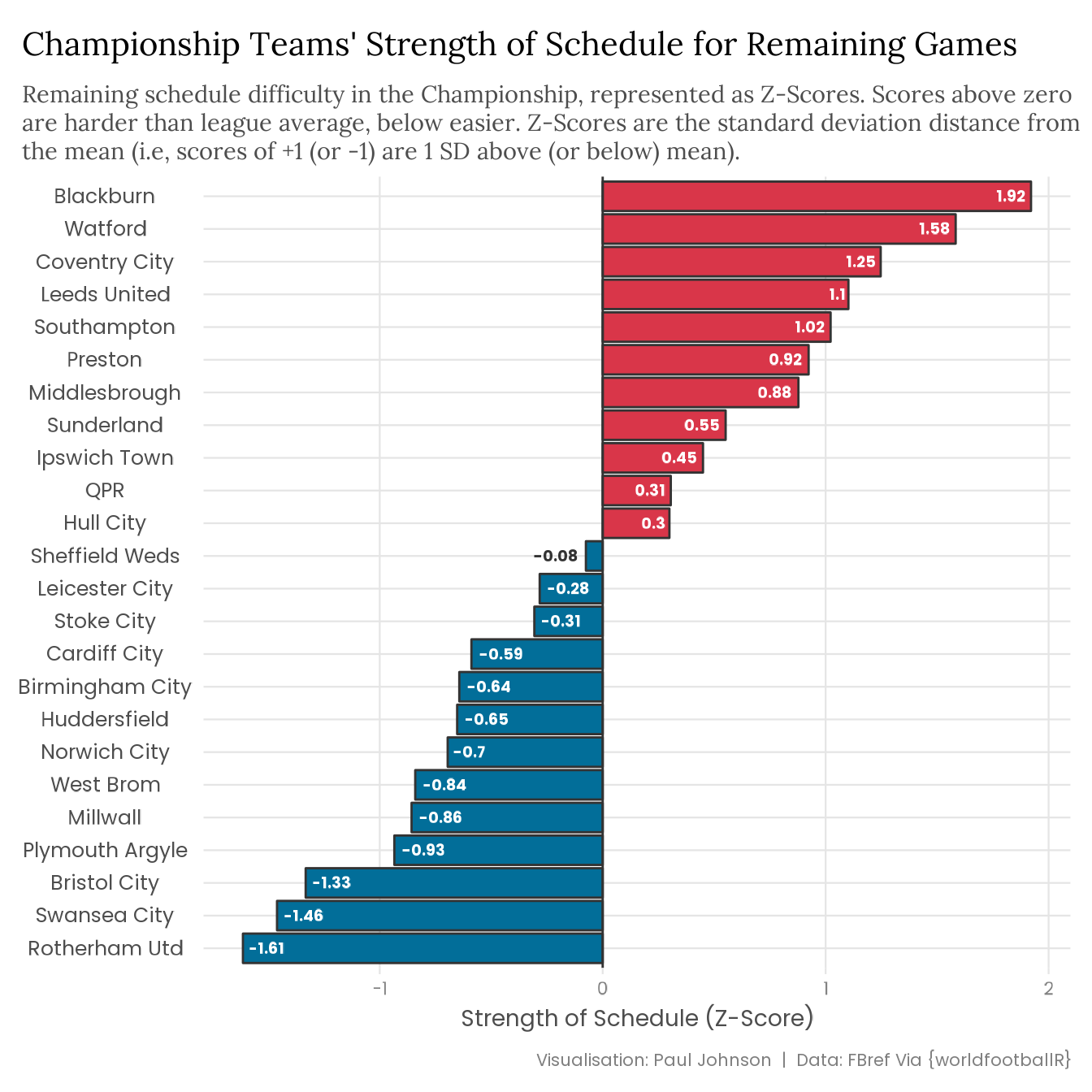
Things don’t look much better when compared to the rest of the league.
Plot Code (Click to Expand)
champ_sos |>mutate(team = forcats::fct_reorder(team, sos)) |>ggplot(aes(x = team, y = sos, fill = sos >0)) +geom_col(colour ="grey20") +geom_hline(yintercept =0, colour ="grey20") +geom_text(aes(label =round(sos, 2),colour =between(sos, -0.25, 0.25),hjust =case_when(between(sos, -0.25, 0) ~1.2,between(sos, 0, 0.25) ~-0.4, sos <-0.25~-0.2, sos >0.25~1.2 ) ),size =5, fontface ="bold", family ="Poppins" ) +coord_flip() +scale_fill_manual(values =c("#026E99", "#D93649"), guide ="none") +scale_colour_manual(values =c("white", "grey20"), guide ="none") +labs(title ="Championship Teams' Strength of Schedule for Remaining Games",subtitle = stringr::str_wrap( glue::glue("Remaining schedule difficulty in the Championship, represented as ","Z-Scores. Scores above zero are harder than league average, below ","easier. Z-Scores are the standard deviation distance from the mean ","(i.e, scores of +1 (or -1) are 1 SD above (or below) mean)." ),width =95 ),x =NULL, y ="Strength of Schedule (Z-Score)",caption ="Visualisation: Paul Johnson | Data: FBref Via {worldfootballR}" )
No problem. Last night I asked my landlord the Championship to increase my rent the gap between the top three and Saints. That’s how much I believe in my Southampton’s grind/hustle.
Limitations
The most significant limitation is that this could be a lot more precise. I suspect the team ratings are the area with the greatest room for improvement. The 70%/30% split between npxGD/90 and npGD/90 is acceptable as a starting point, but a more precise approach to measuring team strengths will make a big difference in the final SOS calculations since the ratings do most of the heavy lifting.
The other major component in the model is how the opponents’ opponents are factored in as a means of weighting team ratings more effectively. I like the approach used here. It is a reasonably simple but effective way to get at this issue. That said, I wonder if the weight given to OR and OOR is ideal. I can’t think of a more robust approach, but maybe there is a better way to do things?
Finally, from a slightly different angle, should the baseline team ratings incorporate the schedules that each team has faced so that they are a more accurate representation of team strengths11? This doesn’t impact the final results of the SOS model, but it would make the team ratings more meaningful.
Summary
Nothing I’ve done here is particularly fancy or impressive, but SOS seems to be an overlooked area of football analytics, so does this at least fill a small gap? I’m sure SOS hasn’t received much attention because it’s just not that interesting, and everyone can live without it, but I fancied having a little play around with it, and here we are.
I can’t think of a better way to validate these results besides the eye test, but looking over the SOS for both the Premier League and the Championship, the results feel approximately correct. With the fitba package, this approach can be applied to past or remaining schedules. It will be little use if you’re trying to measure SOS for the first handful of games in a season, but why would you do that anyway? Stop being a bozo and wait a few games. Regardless, I hope this method can be helpful to someone, even if only inspiring them to come up with something much better because I’m an idiot.
If anyone wants to complain about it being called soccer, then please a) grow up, and b) go look at who first came up with that term.↩︎
I’m not claiming to be an expert in the various ways SOS is calculated in American sports, so if you’re after a detailed literature review, I’m afraid you’ve come to the wrong place.↩︎
I have included notation for each step in building the model, but I have hidden it because it isn’t necessary to understand the methodology. It’s just there for the sickos.↩︎
I mean, clearly, that’s not true. This blog post would not exist if I wasn’t an insufferable bore. But even I have my limits.↩︎
My main reason for abbreviating this is because writing this multiple times (and not messing up the punctuation) was intolerable.↩︎
I’m unsure if my concerns are warranted. I may be overthinking things. Feedback is welcome!↩︎
Functions InTended for footBall Analytics… Yes, I’m an idiot↩︎
The same applies to the top three in the Premier League this season. I care less about giving them credit.↩︎
Look, I know this isn’t true. For a while, the underlying numbers suggested they might be a level below Leeds, Leicester, and Saints. The numbers haven’t had my back for a while now, but I also watched multiple Ipswich games where they never really stood out (though they were pretty good against Southampton on Monday). I know it isn’t true. I’m sure I just watched a bad sample of Ipswich games. Let me live.↩︎
Yes, they probably should, but I also only just thought of this, and I can’t be bothered to go back and fix it right now.↩︎